DEVELOPER’s BLOG
技術ブログ
TensorFlowでVGG19を使ったインスタ映え画像の生成
概要
DeepArtのようなアーティスティックな画像を作れるサービスをご存知でしょうか?
こういったサービスではディープラーニングが使われており、コンテンツ画像とスタイル画像を元に次のような画像の画風変換を行うことができます。この記事では画風変換の基礎となるGatysらの論文「Image Style Transfer Using Convolutional Neural Networks」[1]の解説と実装を行っていきます。
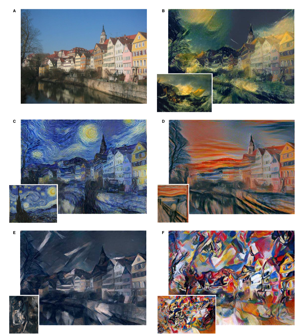
引用元: Gatys et al. (2016)[1]
手法
モデルにはCNN(Convolutional Neural Network) が用いられており、VGG[2]という物体認識のための事前学習済みのモデルをベースとしています。
こちらの図はCNNが各層においてどのようにコンテンツ画像とスタイル画像を表現するか示しています。
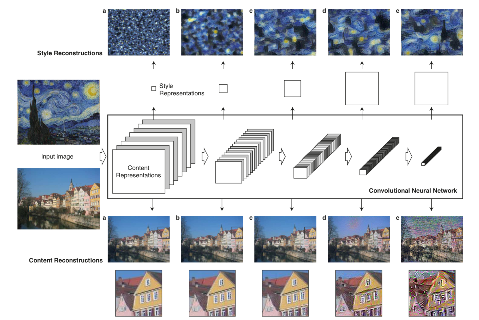
引用元: Gatys et al. (2016)[1]
Content Reconstructions (下段) のa, b, c を見ると入力画像がほぼ完璧に復元されていることがわかります。一方で d, e を見ると詳細な情報は失われているものの、物体認識をする際に重要な情報が抽出されていることがわかります。これは画像からコンテンツが抽出され、画風を表す情報が落とされていると考えられます。よって画風変換のモデルでは画像からコンテンツを捉えるためにCNNの深い層を利用します。
次にStyle Reconstructions (上段) を見てみましょう。a からe はそれまでの各層の特徴マップの相関をもとに復元されています。例えば c は第1層から第3層までの各層における特徴マップの相関から生成されています。こうすることで画像内のコンテンツの配置などによらない画風を抽出することができます[3]。
画風変換のモデルではコンテンツ画像とスタイル画像を入力として受け取り、上記のことを利用してスタイル画像の画風をコンテンツ画像に反映した画像を新たに生成します。
では具体的にモデルの中身を見ていきましょう。
モデルのアーキテクチャ
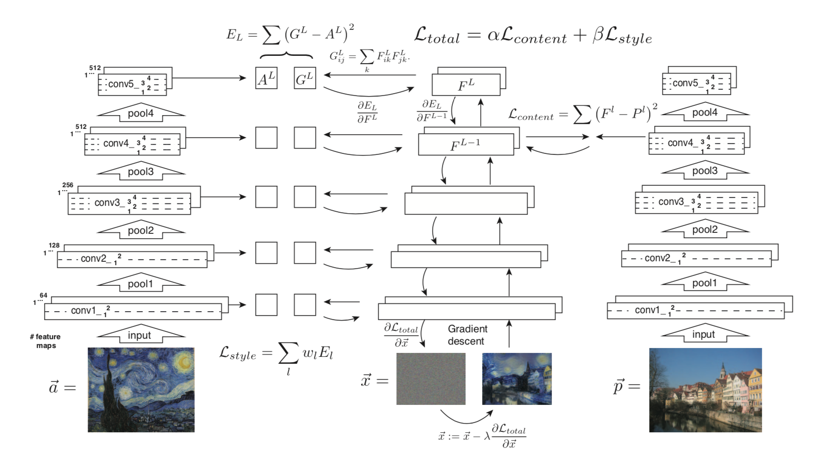
引用元: Gatys et al. (2016)[1]
ここで注意しなければならないことが1つあります。通常、ディープラーニングでは重みが最適化の対象になりますが、今回は重みは固定して生成画像のピクセルを最適化します。
コンテンツ損失
コンテンツ損失はコンテンツ画像と生成画像のVGGのある1層から出力された特徴マップの平均二乗誤差によって計算されます。
スタイル損失
スタイル画像から画風を捉えるためにまず各層における特徴マップの相関を計算します。
最適化
実装
実装にはTensorFlowを用いました。また実装に際してTensorFlowのチュートリアル[4]を参考にしました。
まずは必要なライブラリをインストールします。
import numpy as np
import matplotlib.pyplot as plt
import matplotlib as mpl
%matplotlib inline
mpl.rcParams['figure.figsize'] = (12,12)
mpl.rcParams['axes.grid'] = False
import time
import IPython.display as display
import PIL.Image

import tensorflow as tf
from keras.preprocessing import image
画像を読み込んで配列に変換する関数、テンソルを画像に変換する関数を定義します。
# 画像を読み込み配列に変換し正規化する
def load_image(input_path, size):
    image = tf.keras.preprocessing.image.load_img(input_path, target_size=size)
    image = tf.keras.preprocessing.image.img_to_array(image)
    image = np.expand_dims(image, axis=0)
    image /= 255
    return image


# テンソルを画像に戻す
def tensor_to_image(tensor):
    tensor = tensor.numpy()
    tensor *= 255
    tensor = np.array(tensor, dtype=np.uint8)
    if np.ndim(tensor)>3:
        assert tensor.shape[0] == 1
        tensor = tensor[0]
    return PIL.Image.fromarray(tensor)
このクラスは配列に変換された画像を受け取り、VGG19の各層からの出力を返します。この時点でスタイルの表現に使われる特徴マップはグラム行列に変換されます。
class StyleContentModel():
    def __init__(self):
        # VGG19のどの層の出力を使うか指定する
        self.style_layers = ['block1_conv1', 'block2_conv1', 'block3_conv1', 'block4_conv1', 'block5_conv1']
        self.content_layers = ['block5_conv2']

        self.num_style_layers = len(self.style_layers)
        self.vgg = self.get_vgg_model()
        self.vgg.trainable = False

    def __call__(self, inputs):
        preprocessed_input = tf.keras.applications.vgg19.preprocess_input(inputs * 255)
        vgg_outputs = self.vgg(preprocessed_input)

        style_outputs, content_outputs = (vgg_outputs[:self.num_style_layers], vgg_outputs[self.num_style_layers:])
        style_outputs = [self.gram_matrix(style_output) for style_output in style_outputs]

        style_dict = {style_name:value for style_name, value in zip(self.style_layers, style_outputs)}
        content_dict = {content_name:value  for content_name, value in zip(self.content_layers, content_outputs)}

        return {'style':style_dict, 'content':content_dict}

    # Keras API を利用してVGG19を取得する
    def get_vgg_model(self):
        vgg = tf.keras.applications.vgg19.VGG19(include_top=False, weights='imagenet')
        vgg.trainable = False

        outputs = [vgg.get_layer(name).output for name in (self.style_layers + self.content_layers)]
        model = tf.keras.Model(vgg.input, outputs)

        return model

    # グラム行列を計算する
    def gram_matrix(self, input_tensor):
        result = tf.linalg.einsum('bijc,bijd->bcd', input_tensor, input_tensor)
        input_shape = tf.shape(input_tensor)
        num_locations = tf.cast(input_shape[1] * input_shape[2], tf.float32)
        return result / num_locations
そして合計損失を計算する関数、計算した損失から勾配を計算する関数を定義します。
# 合計損失を計算する
def compute_loss(model, base_image, style_targets, content_targets, style_weight, content_weight):
    model_outputs = model(base_image)
    style_outputs = model_outputs['style']
    content_outputs = model_outputs['content']

    style_loss = tf.add_n([tf.reduce_mean((style_outputs[name]-style_targets[name])**2) for name in style_outputs.keys()])
    style_loss *= style_weight / len(style_outputs)

    content_loss = tf.add_n([tf.reduce_mean((content_outputs[name]-content_targets[name])**2) for name in content_outputs.keys()])
    content_loss *= content_weight / len(content_outputs)

    loss = style_loss + content_loss
    return loss, style_loss, content_loss

# 損失を元に勾配を計算する
@tf.function()
def compute_grads(params):
    with tf.GradientTape() as tape:
        all_loss = compute_loss(**params)

    grads = tape.gradient(all_loss[0], params['base_image'])
    return grads, all_loss
最後に画像の生成を行う関数を定義していきます。
生成画像のベースとなる画像にはノイズ画像を指定しています。ベース画像にコンテンツ画像やスタイル画像を指定するとまた違った結果が得られます。
def run_style_transfer(style_path, content_path, num_iteration, style_weight, content_weight, display_interval):
    size = image.load_img(content_path).size[::-1]
    noise_image = np.random.uniform(-20, 20, (1, size[0], size[1], 3)).astype(np.float32) / 255
    content_image = load_image(content_path, size)
    style_image = load_image(style_path, size)

    model = StyleContentModel()
    style_targets = model(style_image)['style']
    content_targets = model(content_image)['content']

    # 生成画像のベースとしてノイズ画像を使う
    # ベースにはコンテンツ画像またはスタイル画像を用いることもできる
    base_image = tf.Variable(noise_image)

    opt = tf.optimizers.Adam(learning_rate=0.02, beta_1=0.99, epsilon=1e-1)

    params = {
        'model': model,
        'base_image': base_image,
        'style_targets': style_targets,
        'content_targets': content_targets,
        'style_weight': style_weight,
        'content_weight': content_weight
    }

    best_loss = float('inf')
    best_image = None

    start = time.time()
    for i in range(num_iteration):
        grads, all_loss = compute_grads(params)
        loss, style_loss, content_loss = all_loss

        opt.apply_gradients([(grads, base_image)])
        clipped_image = tf.clip_by_value(base_image, clip_value_min=0., clip_value_max=255.0)
        base_image.assign(clipped_image)

        # 損失が減らなくなったら最適化を終了する
        if loss < best_loss:
            best_loss = loss
            best_image = base_image
        elif loss > best_loss:
            tensor_to_image(base_image).save('output_' + str(i+1) + '.jpg')
            break

        if (i + 1) % display_interval == 0:
            display.clear_output(wait=True)
            display.display(tensor_to_image(base_image))
            tensor_to_image(base_image).save('output_' + str(i+1) + '.jpg')
            print(f'Train step: {i+1}')
            print('Total loss: {:.4e}, Style loss: {:.4e}, Content loss: {:.4e}'.format(loss, style_loss, content_loss))

    print('Total time: {:.4f}s'.format(time.time() - start))
    display.clear_output(wait=True)
    display.display(tensor_to_image(base_image))

    return best_image
では実際に画風変換を行ってみましょう。styleweightとcontentweightはそれぞれスタイル損失とコンテンツ損失の重みを表します。
style_path = '../input/neural-image-transfer/StarryNight.jpg'
content_path = '../input/neural-image-transfer/FlindersStStation.jpg'
num_iteration = 5000
style_weight = 1e-2
content_weight = 1e4
display_interval = 100

best_image = run_style_transfer(style_path, content_path, num_iteration, style_weight, content_weight, display_interval)
結果
コンテンツ画像とスタイル画像はこれらの画像を使いました。
コンテンツ画像
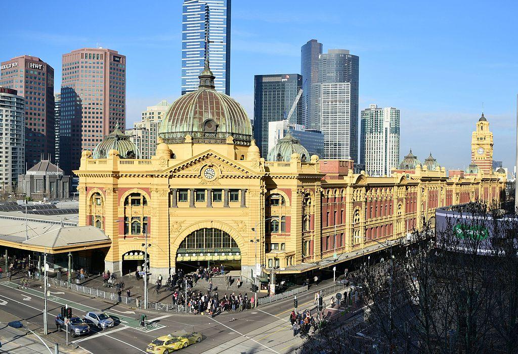
引用元: https://commons.wikimedia.org/wiki/File:Flinders_Street_Station_3.jpg
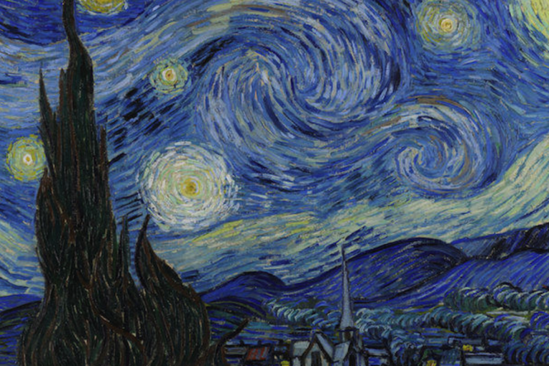
スタイル画像
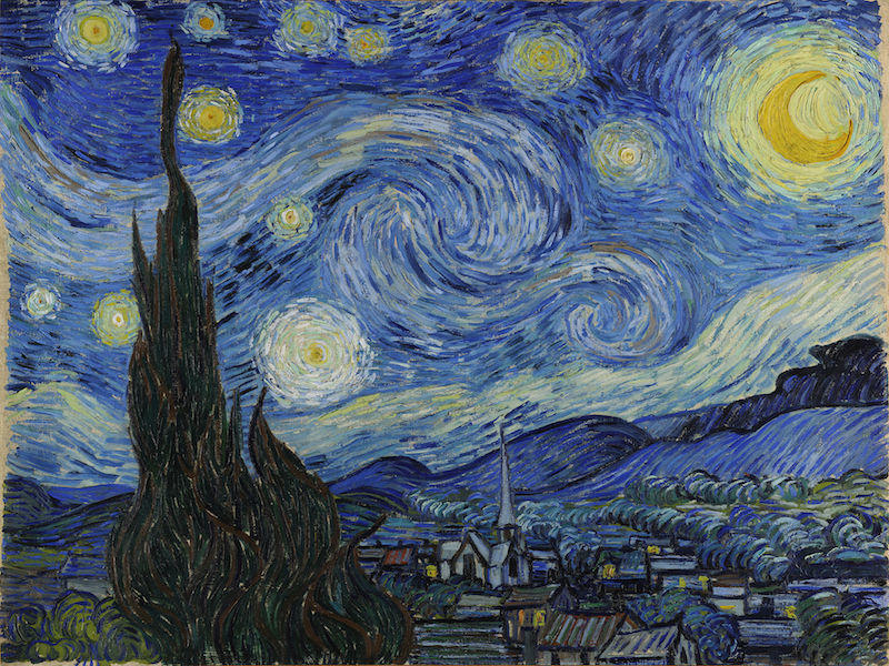
引用元: https://commons.wikimedia.org/wiki/File:Van_Gogh_-_Starry_Night_-_Google_Art_Project.jpg
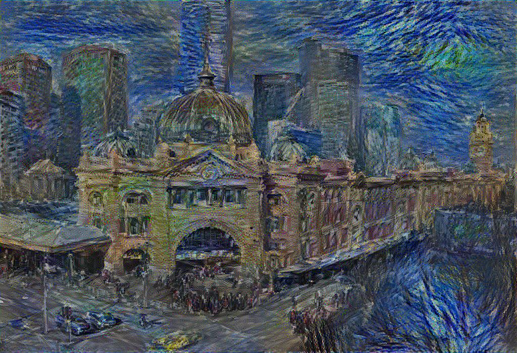
上記のコードを走らせて生成した画像がこちらになります。
スタイル損失とコンテンツ損失の重みを変えて4種類の画像を生成しました。
- \(\alpha = 10, \beta = 10^{-2}\)
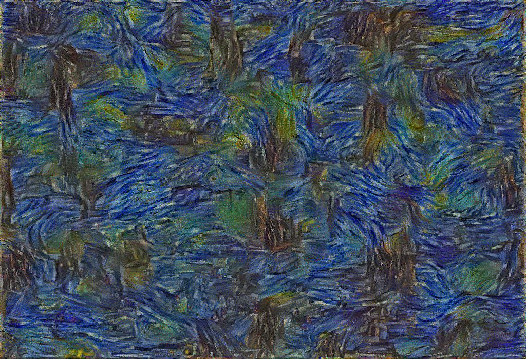
- \(\alpha = 10^{2}, \beta = 10^{-2}\)
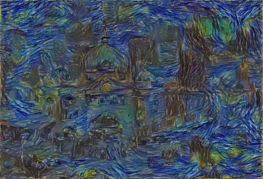
- \(\alpha = 10^{3}, \beta = 10^{-2}\)
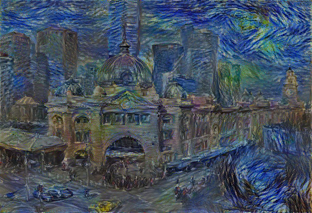
- \(\alpha = 10^{4}, \beta = 10^{-2}\)
まとめ
今回は画風変換の基礎となる論文の解説と実装を行いました。ベース画像やパラメーター、VGGのどの層の出力を使うかなどによって違った結果が得られるので色々といじってみるのも面白いかもしれません。またこの論文以降にも画風変換の研究が進められていますので、それらを試す助けになればと思います。
参考文献
[1] Image Style Transfer Using Convolutional Neural Networks
[2] Very Deep Convolutional Networks For Large-scale Image Recognition
[3] Texture Synthesis Using Convolutional Neural Networks
[4] TensorFlow Core: Neural style transfer
Twitter・Facebookで定期的に情報発信しています!
Follow @acceluniverse
関連記事
ディープラーニングを使って、人の顔の画像を入力すると 年齢・性別・人種 を判別するモデルを作ります。 身近な機械学習では1つのデータ(画像)に対して1つの予測を出力するタスクが一般的ですが、今回は1つのデータ(画像)で複数の予測(年齢・性別・人種)を予測します。 実装方法 学習用データ まず、学習用に大量の顔画像が必要になりますが、ありがたいことに既に公開されているデータセットがあります。 UTKFace というもので、20万枚の顔画像が含まれています。ま
概要 自分に似合う色、引き立たせてくれる色を知る手法として「パーソナルカラー診断」が最近流行しています。 パーソナルカラーとは、個人の生まれ持った素材(髪、瞳、肌など)と雰囲気が合う色のことです。人によって似合う色はそれぞれ異なります。 パーソナルカラー診断では、個人を大きく2タイプ(イエローベース、ブルーベース)、さらに4タイプ(スプリング、サマー、オータム、ウィンター)に分別し、それぞれのタイプに合った色を知ることができます。 パーソナルカラーを知るメ
はじめに この記事では物体検出に興味がある初学者向けに、最新技術をデモンストレーションを通して体感的に知ってもらうことを目的としています。今回紹介するのはAAAI19というカンファレンスにて精度と速度を高水準で叩き出した「M2Det」です。one-stage手法の中では最強モデル候補の一つとなっており、以下の図を見ても分かるようにYOLO,SSD,Refine-Net等と比較しても同程度の速度を保ちつつ、精度が上がっていることがわかります。 ※https:
はじめに まずは下の動画をご覧ください。 スパイダーマン2の主役はトビー・マグワイアですが、この動画ではトム・クルーズがスパイダーマンを演じています。 これは実際にトム・クルーズが演じているのではなく、トム・クルーズの顔画像を用いて合成したもので、機械学習の技術を用いて実現できます。 機械学習は画像に何が写っているか判別したり、株価の予測に使われていましたが、今回ご紹介するGANではdeep learningの技術を用いて「人間を騙す自然なもの」を生成する